Distributional effects of an increase in the Carbon Tax within a partial equilibrium framework- the case of Sweden

Ingvar Nilsson & Anders Wadeskog

1998-06-01

This paper was prepared for EC Environment and Climate Research Programme (1994-1998): Research Theme 4 - Human Dimensions of Environmental Change
Environmental Fiscal Reform(ENV4-CT 96-0228)

Fiscal measures aimed at reducing the demand for environmentally sensitive goods and services (ESGS), has come to be seen as a necessary tool for moving in a more sustainable direction. Changes in prices, brought about by taxes and subsidies, will almost always have distributional effects.

The distributional effects of fiscal measures in the environmental area have had to take a back seat, for many years, in relation to the pros and cons in terms of the environmental effects. This is perhaps not surprising, as the chief interest from economists, with regards to market based instruments for the environment, have been in the efficiency properties of these instruments.

However, in recent years, the distributional effects have received increasing attention in many countries. In most countries, ESGS such as petrol consumption, claim a higher share of total expenditures for low income households than it does in higher income households. This implies that a fiscal reform aiming at increasing, for instance, the price of petrol, will affect the total expenditures of low income households more than the total expenditures of high income households.

This is more or less evident from just looking at the expenditure patterns in different countries. The changes in prices brought about by the tax changes will of course alter the composition of the expenditures. Households will adapt its expenditure to reflect that some goods and services have become relatively more expensive. Depending on the price effects between substitutes, some reallocation of expenditures would be expected. This adds another dimension to the effect of the increase in the prices of ESGS in different types of households.

A fiscal reform on ESGS is mainly argued along efficiency lines, i.e. that the price changes introduced are corrective in the sense that these goods and services can be seen as having been subsidised so far. Prices have not included the true cost of consuming them. The tax, or levy, can be seen as an attempt to correct this implicit subsidy.

There is also another side to this kind of tax or levy. As other taxes, it generates revenues. In many cases, taxes are introduced for no other reason than to generate revenue, but a corrective environmental tax does not primarily have this purpose.

Revenues can, however, be used in different ways. They could, for instance, be targeted to increase the efforts in the environmental field in general. It is also possible, and probably necessary, to consider using the revenues to reduce other taxes. On the one hand this could be seen as a way of keeping the total tax pressure constant. On the other, this has been introduced in the debate as a possibility to substitute taxes that have greater distortionary effects. This is part of what the debate on the, so called, double dividend has focused on. Another possible use of the revenue is of course to alleviate the expected distributional effects of the fiscal measures on ESGS. Most economists would prefer some kind of lump sum transfer to counter act the distributional effects, but this is perhaps not possible in most countries.

In this paper the focus is on the distributional effects of a change in the carbon tax for Sweden. The analysis is done from a demand side point of view, i.e. in a partial equilibrium framework. The tax and revenue side of the change is also modelled in order to be able to look at possible compensations and the changes in tax revenues.

The results are not really surprising. A doubling of the carbon tax will have negative distributional effects regardless if one look at expenditure group, disposable income groups, or regional groups.

A compensation through a decrease in the VAT has been suggested as a remedy for these negative effects. A revenue neutral decrease in the VAT will change the levels of, but not erase, the losses. All household categories have to be compensated in order to achieve the same welfare as before the change. The less well off households will suffer more than the more well off households.

The net loss due to the tax change should naturally be viewed against and compared to the presumed gain from a better environment. This is really the purpose of the tax change in the first place.

The calculations in this paper is based on a Linear Almost Ideal Demand system model. It has been estimated for durable goods as one category and then 12 aggregated non durable goods, where it is assume that the household first allocates its income between durable and non durable goods and then within the non durable goods.

The estimations are based on both macro data and micro data. The price elasticities are based on the data from the national accounts on final private consumption, while the income/budget elasticities are based on data from a household budget survey. This combination of time series and cross section is really a second best solution compared to having a series of expenditure surveys.

A household budget survey is the only source for doing distributional analysis of consumption and expenditures. Most countries make household budget surveys, with varying intervals. The trend in the member states seem to be towards having annual expenditure surveys with reduced samples, compared to the intermittent surveys. This is promising for future analysis. The classifications used, in terms of household types, in the comparative tables published by Eurostat have apparently shifted from incomes to expenditures. And to further complicate matters the expenditure classification is not in deciles or quintiles, but in expenditure groups in relation to the mean expenditure. This shift from income to expenditure is probably mostly due to the poor income estimates in many countries.

Looking at the possibilities of using the national accounts data and household budget survey data as it is compiled at Eurostat poses some interesting problems when using these kinds of data for distributional analysis.

One is due to the problem of specifying what constitutes an economically weaker household. Traditionally, the use of income as an indicator of the level of resources at a households disposal has been rather straight forward. The relevant base for the evaluation in terms of adult equivalents have, on the other hand, been the subject of much debate. How does the change in focus to expenditure groups alter the possibilities of finding vulnerable groups? Does a lower level of expenditures really mean that the household is economically weaker than an otherwise comparable household with a higher level of expenditure?

The other problem has to do with the discrepancies between private consumption as it is calculated in the national accounts and private consumption as it comes out in the household budget surveys. The former should ideally build on the latter, but this is seldom the case. There are major differences between the two measures of total private consumption. The household budget survey in general gives lower over all figures. This is important to be aware of when combining the two types of accounts.

Although the papers main objective is to present the results of simulations on an increase in the tax on carbon we will discuss these two problems briefly. It is, however, not within the scope of this paper to do any deeper analysis of these issues.

In the original design of the project, the distributional analysis was to be done according to income quintiles. The potential regressiveness of fiscal measures was to be evaluated for different income quintiles. This was a natural starting point as most Statistical offices and also the pre 1988 Eurostat compilations published expenditure data with some sort of income groupings.

The (ca) 1988 compilations did not follow this route. Instead it used an expenditure based grouping of households. In the relevant tables it uses Total expenditures per adult equivalent instead of the income groups. The groups are < 0.4, 0.4-0.6, 0.6-0.9,0.8-1.2,1.2-1.6 and >1.6 of the mean total expenditures per adult equivalent.

As mentioned above, this approach causes some problems.

- It makes the idea of finding the economically weaker households and studying the impact on them, more difficult. It is definitely easier to argue that a household with a low income is economically weak or vulnerable, than to argue that a household that consumes less is economically weaker. In order for the argument to hold, one has to assume that there is a strong relationship between income and expenditure.

- There is a possibility that the households that appear weak, by the expenditure classification, in fact are frugal, i.e. they do not maximise consumption. This will of course always be the case when using expenditure data in itself, but with the classification by income groups, the frugal households would be in the right category. The distribution of frugal households within each income group is probably not symmetric, but that is another issue.

It was possible to use the data from the Swedish expenditure surveys to compare the groupings on income or expenditure and this enabled at least a tentative picture of the relationships between the two ways of grouping households. Perhaps Sweden is not a good case given the tax/transfer schemes and the level of public provision or financing of consumption in place in the late 80's, but it is an interesting comparison nonetheless.

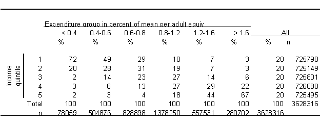
In the table below, based on the 1992 expenditure survey, households have been tabulated according to income quintile of disposable expenditure (rows) per adult equivalent and to expenditure as proportion of mean income (columns) per adult equivalent. The numbers are rounded percentages and show the distribution over the income categories within a certain expenditure category.

It is apparent that the hoped for clustering of households on the diagonal is not present. Although a large percentage of the households in the lower expenditure groups also are the households in the lower income groups, the distribution is far from ideal. 5% of the households in the lowest expenditure groups belong to the top two income categories and 6% of the households in the highest expenditure group belong to the two lowest income groups.

Looking at the same distribution in a chart, the distributions appear more clearly.

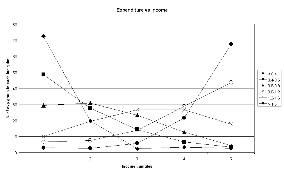
The definition of weak or vulnerable household is not self evident. Other factors than income certainly influence the real or perceived vulnerability of a household. But income is most likely preferable to expenditures, especially if these show a less than hoped for correlation with income groupings.

All in all, the reliance on the expenditures instead of incomes makes it complicated to analyse the distributional effects of fiscal measures as, for one thing, a group of household may (mistakenly?) be classified as poor or weak, when they are actually frugal and may be quite well off. To further complicate matters, although this is less likely in a survey of this scope, it may also be that they are frugal for environmental reasons, i.e. they minimise consumption in general and consumption of ESGS in particular. If this is the case, one could even envision a situation where fiscal instruments could cause a Giffen-type of situation with the effects of the tax working in the wrong direction.

The estimation model used is based on the assumption of households having preferences that are weakly separable over time between durable and non durable goods. This means that it is possible to view household demand for non durable goods as a function of prices and total expenditure on non durable goods in itself.

Prices on durable goods will affect the demand for non durable goods through the expenditure share on durable goods, i.e. a constant proportion of expenditure, regardless of the level. The rest is used on non durable goods.

The Linear Almost Ideal Demand system has been used to estimate the demand system for non durable goods. In this model, the expenditure shares for each group of goods is specified as a linear function of the prices (log) and real expenditure (log) on non durable goods.

where

share of total expenditure on non durable goods that is spent on good i.

price index for good j

P = price index for non durable goods, approximated by Stones price index where is the average expenditure share for good j

y= total expenditures on the K different non durable goods

= error term

= the estimated parameters

has been specified as in the estimations, where is a vector of household characteristics.

The uncompensated price elasticities in the Slutsky matrix can be written as

where

if i=j and 0 otherwise

The budget elasticities can be written

In the estimates, the adding up condition , i.e. , the homogeneity condition as well as the symmetry condition is imposed.

As stated earlier, the model is estimated on a combination of macro and micro data. The macro data used are the final private consumption by purpose, from the national accounts. These are annual figures for the period 1970-1995. The macro data are used to estimate the price elasticities . The micro data used come from the 1992 Household Budget Survey (HBS). This is used to estimate the budget shares and gives the base for the distributional analysis.

Detailed expenditure surveys has a thirty year history in Sweden. Since the late 60’s there has been half a dozen large scale expenditure surveys that cover some 200 goods and services. The methods and instruments used have varied slightly over the years, depending on specific purposes. For instance, the inclusion of detailed surveys of the expenditure on food stuffs, more or less emphasis on distribution within households in clothing expenditure, etc.

The 1992 survey was the last (so far) full scale survey covering a year and with a large sample. As of 1995 the survey is supposed to be carried out on a continuos basis with a reduced sample of app. 200 households per month participating. The move to an annual survey is in line with the development in the majority of the member states.

The modelling is based on the 1992 HBS. This survey was based on a sample of 6000 households of which 3806 participated in all moments of the survey. They kept an expenditure log of everything purchased over a 4 week period. In addition to this there is an interview in which background data on the household is collected, as well as data collected from registers, mainly on incomes.

Using a combination of micro and macro data it would, of course, be an advantage if the results obtained in the two sources in terms of total expenditure/consumption were roughly the same. It is furthermore something that would be expected as one of the original expressed aims of the HBS was to provide a basis for compiling the private consumption part of the national accounts.

Ideally, a yearly HBS would be used to assist the national accounts on:

- the composition of private consumption, i.e. the levels of each commodity group.

- parts of the industry-commodity matrix, that is used to allocate industry output (e.g. from sales data) to goods and services purchased.

- the first forecasts of the private consumption part of GDP, i.e. on the changes for the 1:st quarter.

- subsequent revisions of GDP and private consumption.

Private consumption, and the different GDP components are basically calculated on the changes in the period. This means that the absolute levels of total expenditure as it appears in the HBS is not really of any greater interest. Basically, the incremental approach is one way of constructing the accounts in order to achieve consistency in the series.

In some countries, the HBS is seen as a source for independent estimates of the levels of private consumption. This is however somewhat controversial as the levels in the national accounts reflects the base levels set a long time ago as well as the skills in establishing the growth rates in a single period. Differences in the levels predicted from the accounts and from HBS will differ by default and this is probably seen as an argument not to put to much of an emphasis on the totals and levels of the HBS. There is of course no way of concluding that one estimate is more true than the other - although the national accounts figures are consistent with other economic indicators.

The final consumption in the national accounts (NAPC) is based on many sources - of which the HBS is one, although insignificant, source. The last time the HBS was put to any greater use in the national accounts in Sweden, was when using the 1978 survey to reset the levels of private consumption in the early 80's. Apart from a few exceptions, these are still the base levels used in the national accounts.

It is well known that NAPC and total expenditures as they come out in the HBS differ. According to a survey by Eurostat, the discrepancy for total consumption is around 30%, of which 2/3 comes from differences in population, concepts and definitions and the rest comes from underreporting of different sorts. The differences for some countries are presented in the table below.

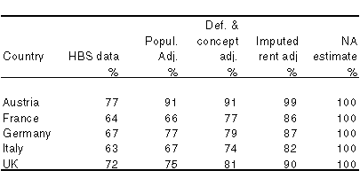
The differences in population stems from the fact that HBS survey private households. This means that it does not include persons living in institutions or foreign tourists. Both included in the NAPC. It also comes from the differences in the age groups surveyed in the HBS. In Sweden there is an age limit of 75 in the HBS while the NAPC covers consumption of all, regardless of age.

The differences in definitions and concepts are due to the different treatment of a series of expenditure types. Among these are:

Consumption of household own production, benefits in kind, insurance, hiring/leasing, gifts and transfers, equipment and clothing needed for work, capital expenditure etc.

The major part of the difference in concepts and definitions has to do with the imputation of the rent of housing.

An adjustment of the HBS to cater for these differences, will bring the totals closer, but there will still be discrepancies in different goods categories. In the table below, the discrepancies for single goods can range from 20% up to 140% comparing other goods n.e.c for Italy and Austria. Or between 40% and 200% looking over all goods in the Austrian expenditure survey.

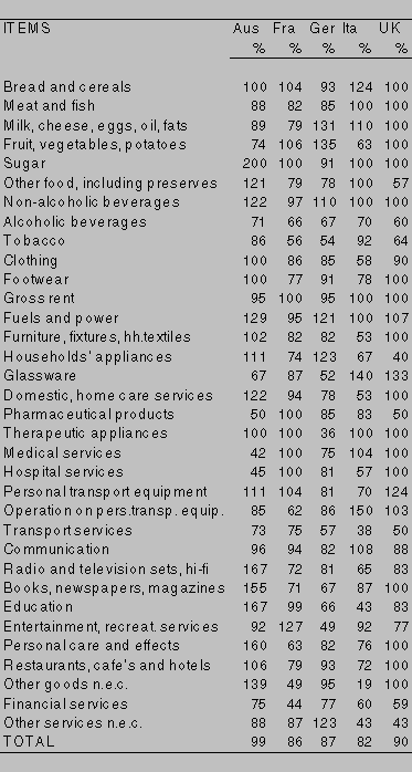
For the goods most of interest here, i.e. goods like operations on personal transport equipment, transport services, fuels and power, etc., it is apparent that the discrepancies vary from over- to underestimation. Transport services are all lower while fuels and power are mostly overestimated.

In the case of Sweden the comparison between the 1992 HBS, adjusted for population differences, and the national accounts show the following pattern for some of the relevant goods:

One of the problems with these differences is that the expenditure shares estimated from macro and micro data will come out differently. The expenditure share for transportation (i.e. public transports) will for instance be much lower than the expenditure share for the same commodity in the macro data, especially using the unadjusted figures from the HBS. The same applies to household energy (i.e. public transports) expenditure category. The expenditure shares of Petrol and other costs for personal transportation (that has been aggregated into Car Maintenance in the model) will be higher in the micro data.

The demand system has been estimated for the following 12 categories of non durable goods:

Leisure/Culture, which includes all leisure goods, charter tours, hotels, restaurants, private education entertainment etc.

Literature, i.e. books and magazines

Publ transp/communication, i.e. travel by rail, air or water, telecommunication, mail

Car maintenance, i.e. fuel, repairs, parking etc

Household fuel, i.e. gas and other fuels

Household Services, i.e. repairs, washing and cleaning, child care, hair dressers etc.

Other, includes financial services and health care

This is not an ideal aggregation. One would probably have wished for a better disaggregation of the transports and some of the components now in the leisure/culture categories. The main reason for choosing this classification is one of quality of data. Initial tests with more disaggregated classifications gave very poor estimates. Another reason is, of course, comparability with previous estimates.

The uncompensated price elasticities, evaluated at the mean expenditure shares (in the macro data), are by and large of the expected sizes and signs. The own price elasticities are marked on the diagonal of the split matrix. The only own price elasticity with a positive sign is that of literature, which is a notoriously difficult commodity in the national accounts.

The own price elasticity of car maintenance, i.e. mainly petrol, is -0.06. This means that a 1% increase in the price will reduce the demand by 0.06%, i.e. that petrol is a very price insensitive good. This elasticity is lower than those produced with similar methods in other analysis where it usually is set to above 0.1 with a long run elasticity closer to the one found in this study. A low elasticity is also given for household energy, -0.01.

The higher own price elasticities are found for leisure (-1.144) and clothing (-1.095).

Alcohol has an unexpectedly high own price elasticity of -1.033.

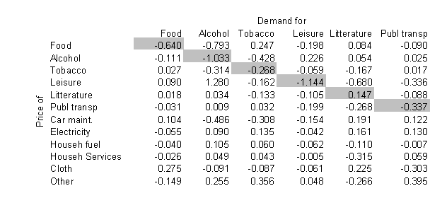
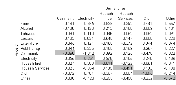Car maintenance and public transports are substitutes, as the cross price elasticities are positive. A 1% increase in car maintenance price will increase the demand for public transport by 0.1%.

The same relationship exist between household fuel and electricity, where a 1% increase in the price of electricity will increase the demand for household fuel by 0.578%.

Turning to the budget elasticities (evaluated at the mean expenditure shares from the micro data) there is a clear pattern with Alcohol, Leisure, Household services, Clothing and Other commodities being seen as luxuries (i.e. with a budget elasticity of > 1). Food, car maintenance, Electricity and Household fuel are necessities with an elasticity of <1. The estimation shows Tobacco to be a necessity in these terms.

The elasticities are evaluated at the mean expenditure shares and are interpreted as the relationship between a 1% increase in expenditure on non durable goods and the percentage change in demand for the different groups of goods.

The micro data also allows for a grouping of the household according to different household characteristics, such as demographics, socio-spatial dimensions, housing etc.

Looking at the share for food expenditure this is positively related to the presence of smaller children while expenditure on alcohol and tobacco is negatively related to the presence of smaller children.

Living in a big city decreases the expenditure share for car maintenance and for electricity, while living in the rural north increases these expenditures.

Living in a rented apartment decreases the expenditure share for electricity and car maintenance while living in a owner occupied dwelling increases the shares expenditure shares.

The expenditure share for car maintenance decreases with increasing socio-economic ranking and that of clothing and leisure goes the other way.

It is well worth noting that the expenditures shares, as they come out of the 1992 HBS, are not very regressive in the ESGS - especially when viewing them by income quintiles.

The basic idea in the simulations is to use the estimated model to predict an expenditure system for the 1995 tax system. This is then used as a baseline to simulate the effects for different household types of a tax increases on CO2. In one scenario without any compensation, and in another, with compensation in the form of a decrease in the VAT, that is set to be revenue neutral in terms of the total revenue collected.

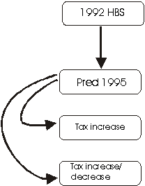
The changes in prices through the changes in the tax system between 92 and 95 for the aggregated expenditure categories is handled in the following way.

where:

the number of homogenous goods, from a tax point of view, in expenditure group i

expenditure share for good k in expenditure group i.

VAT rate for good ik (the rate on the price excluding the VAT). M=0 for 1992 and 1 for 1995

Tax rate for good ik (some taxes are recalculated as value relate taxes although they are in actual case unit taxes) the rate is calculated as the rate on the price excluding the tax. M=0 for 1992 and 1 for 1995

The prices in the 1992 system is set to 1 which means that the price for good iin the 1995 tax system is . These new prices are also used to calculate a new price deflator for total expenditures on non durable goods.

The value related taxes are calculated in the following way

where

For alcohol and tobacco has been calculated as the relation between the tax revenues and the reported total expenditures/sales. The following table lists some of the tax rates for relevant goods. The CO2 tax was 0.34 Sek per Kg in 1995.

The unreduced VAT rates was 25% for the 92-95 period. In 1992 there was a reduced VAT rate of 18% on food, personal transports, hotel and restaurants. In 1995 the VAT for food was 21% and on Hotel and personal transports, 12%.

The tax exempt goods in the 1992-95 period were, among other, apartment rents, housing interests, insurance premiums, health care, education and social care, some cultural goods and services, daily papers, prescribed medicine and packaged holidays travels.

The taxes paid by the household in VAT and other consumption taxes (OT) are calculated in the following way, where the expenditure shares within each expenditure category (incl. durable goods) is set at the 92 level.

for m= 0,1

Using the calculated baseline for 1995, a doubling of the carbon tax is introduced. This will produce a new expenditure mix that will change the amount different households pay in taxes.

The same procedure is repeated, but with a compensating tax decrease in the VAT. The level of this decrease is set to produce roughly the same tax revenues as before the introduction of the raised carbon tax.

The evaluation in terms of the effects for the household is done through the taxes paid and the implicit tax rate for different household types as well as through an estimate of the compensated variation, i.e. the increase in income that different household types would need to return to the level of welfare they had before the change in taxes. The larger the compensated variation, the more the households lose on the tax reform.

The calculation of the compensation amount that would be needed, as a lump sum transfer, in order to for the household to retain its pre-tax welfare is calculated by looking at the expenditure that the household would need with the new set of prices (p) to reach the utility level they had in 95 with 95 prices - CV=.

Using a 2:nd order Taylor approximation this can be written as:

where is a vector of Hicksian demand functions.

can be calculated as the ratio between expenditures and prices over each goods category under the 95 tax system.

is a matrix of compensated own- and cross price elasticities that are calculated in the Linear Almost Ideal Demand system as:

In the simulation results below, the effects of the increase in the carbon tax, as such, are separated from the case where the increase in the carbon tax is offset by a decrease in VAT. The decrease in VAT is just above 6%, or roughly 1.5 percentage points of the full VAT.

The uncompensated increase in the Carbon tax increases the indirect tax paid per adult equivalent and the implicit tax rate, for all groupings. There are however differences.

Looking at the effects over the income per adult equivalent quintiles, the already regressive implicit tax rate get more regressive as the percentage point increase for the higher quintiles are lower than that for the lower quintiles.

The loss in real income, the Compensated Variation, ranges from just over 2000 SEK per household in the lower quintiles to close to 2500 SEK for the highest quintile. Setting this in relation to the expenditure per adult equivalent in the different groups, the lower quintile lose over a percent of their expenditure per adult equivalent in terms of real income while the highest quintiles loses below 1 percent.

Looking at the Eurostat classification according to relation to the mean expenditure per adult equivalent, the distribution becomes more extreme. The implicit tax rate ranges from close to 20% down to just under 14% in the base case. With the increase in the carbon tax this difference is increased with the lowest expenditure groups getting an increase of .8 percentage points and the highest group only getting a .4 percentage point increase.

The losses in real income, measured in relation to their expenditure per adult equivalent show substantial differences. It is almost a 100% difference between the lowest and the highest group.

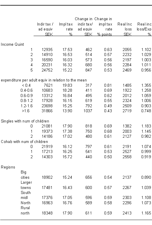
Looking at household types, both singles and couples with children are less hurt by the increase than those without children. The implicit tax rates for singles is generally higher than for couples. The loss in real income in relation to the expenditure per adult equivalent is also higher for singles, with or without children, than for couples with or without children.

The regional perspective indicates that households in the rural north of Sweden will lose more from the increased tax than households in the south. Households in the big cities are best off with a real income loss in relation to expenditure that is well below 1 percent.

In the table below, the results from the simulation with a reduction in the VAT is presented.

The general picture is that the decrease in the VAT benefits those that spend most. The households that actually benefit, in terms of having to pay lower taxes over all, are those in the highest two expenditure groups. This effect does not show up in the income quintiles. There is an increase in the implicit tax rate for most groups, regardless if one look at them from income, expenditure, demographics or a regional perspective.

It is well worth noting the differences in results depending on the choice between expenditure or income grouping of the households. The expenditure grouping gives a sharper regressive effect than the income grouping. Maybe Sweden is a bad case for making these kinds of comparisons, but it is probably wise to interpret the effects received when using the expenditure groupings, with caution.

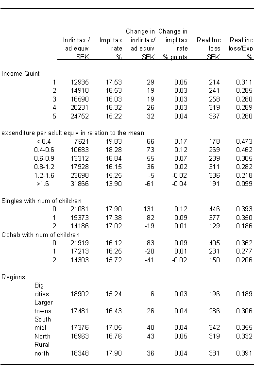
The compensation through VAT increases the relative loss for childless singles and couples in relation to those with children as they have relatively high increases in their implicit tax rate.

The loss in real income is, of course, smaller but still visible. The regional distribution of these losses goes increasingly in favour of the big cities.

The interesting question is how these welfare losses due to the price changes are counterbalanced by other effects. It is not possible to analyse the over all effects in the economy within the present framework, i.e. employment effects and efficiency gains are outside the partial equilibrium analysis.

However, the main purpose of the carbon tax is to reduce emissions. Naturally, this is an expected benefit that should be set against the welfare losses appearing in the analysis.

In the following table the changes in total volumes for the most relevant goods are presented.

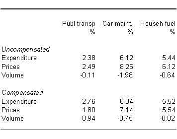
The close to 2% reduction in car maintenance (to a large extent petrol) in the scenario without a compensating VAT reduction will produce a reduction by app. 90 million litres of petrol. The question is how large a reduction in CO2 emissions this, and other reductions in fuels, will produce, both indirectly in the refining process and directly in the use of the fuel.

The analysis of the distributional effects of an increase in the tax on CO₂ gives the expected results. A environmental fiscal reform designed the way presented here will have negative distributional effects. Compensating these effects by offsetting reductions in VAT, is not really possible. This is, of course, not an argument that it is impossible to compensate specific groups that lose in the reform. It is more of an argument for being specific as to how one defines these groups on the one hand, and the need for targeted compensations rather than depending on general measures such as lowering VAT, on the other.

Many factors have been left out of the analysis, as this is a demand-side analysis. The effects on the supply side of the economy could potentially be offsetting, although results using CGE-models for Sweden are not very optimistic on this point.

On a methodological note, this and other similar analysis points to the possibilities of making more use of micro data for analysing sustainability questions from a distributional point of view. To most readers, this kind of analysis will always be a black box that turns out results that may theoretically correct but empirically impenetrable. That is probably inescapable.

However, using these types of simulations will help in addressing the distributional questions at issue. The results may be debated but the focus of the debate will be on distributional issues otherwise neglected.

Much more could probably be done if the micro data used were more easily accessible. With more independent estimations and simulations the distributional questions could be brought further into the policy arena. In a European Community perspective, the comparability issues will always be problematic but also something that is at the heart of much statistical work in the community. Harmonisation is usually at the top of the agenda, and these are problems that should be possible to solve, more or less satisfactory. The present design of the compilation of expenditure surveys, with the expenditure groupings replacing the income groupings, is unfortunately an example of a less satisfactory attempt.